

Matplotlib is a widely used Python package for data visualization. As a powerful 2D plotting library, it allows you to input arrays of numbers and plot the data in various graphical representations, including bar graphs, histograms, scatter plots, and line plots. Particularly, when dealing with graphs that contain multiple lines of varying colors, legends play a crucial role in clarifying the meaning behind these color-coded lines. In this tutorial, we will learn how to add a legend to a Matplotlib plot in Python and customization of legends, thereby enhancing the overall clarity and interpretability of your graphs. To further expand your understanding of Python programming, don’t hesitate to explore additional tutorials available at Python Programming Tutorials.
Let’s delve into the details of how you can create, display, and perform various actions with legends.
Basic Introduction to Legends
A legend serves as a crucial component within a graph, providing valuable graphical representation and information about the elements present in the plot. It helps to identify and differentiate between different data series or plot elements in the graph. Typically, a legend consists of labels or markers that correspond to distinct data categories or plot elements, along with a description or key that explains what each label or marker represents. For instance, in a line plot, each line represents a distinct data series, which can be appropriately labeled within the legend, thereby enabling the viewer to understand which line represents which data. Similarly, in a scatter plot, distinct markers or colors may represent different categories of data, and the legend helps to decode these markers or colors.
Python, being a popular programming language for data visualization, offers powerful libraries such as Matplotlib that facilitate the creation of legends, thereby providing the visual representation of plot elements. In this article, we will explore the concept of legends in data visualization using different types of plots and datasets. Let’s get started!
Adding Legend to Matplotlib Plot
Matplotlib provides a legend() method that allows you to describe what the different lines on a graph represent. To begin, import the Matplotlib library and define the values for the x and y coordinates. Then, pass the coordinates of the graph you want to plot, along with a label indicating what that line represents, to the plot() function. Finally, use the plt.legend() command to add these labels as a legend on the graph. This is the simplest way to add legends to your plot.
To add a legend to a Matplotlib plot in Python, follow these steps:
- Ensure you have imported the
matplotlib.pyplotmodule. - Before plotting, assign labels to each dataset or line by using the
labelparameter within the plotting functions. - After creating the plot, call the
legend()function to display the legend on the plot. Optionally, you can specify the location using thelocparameter, which accepts values such as ‘upper right’, ‘lower left’, etc., or you can use thebbox_to_anchorparameter for a more precise location. - To customize the legend further, you can modify attributes such as font size, background color, frame properties, and more.
- To show the plot with the legend, use the
show()function or save the plot usingsavefig().
Following these steps allows for the seamless integration of a legend into your Matplotlib plot, enhancing its interpretability and visual appeal.
import matplotlib.pyplot as plt

#initialize data
x = [1, 2, 3, 4, 5]
line1 = [1, 2, 3, 4, 5]
line2 = [1, 4, 9, 16, 25]

plt.plot(x, line1, label='x')
plt.plot(x, line2, label='x^2')

# Function add a legend
plt.legend()

# function to show the plot
plt.show()
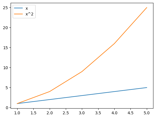
In the above example, we plot two lines with different labels i.e., x and x^2. The plt.legend() command automatically creates a legend based on the provided labels, indicating what each line represents. Finally, the plt.show() function displays the plot with the legend. You can also customize the labels in the legend of a Matplotlib plot as shown in code below.
import matplotlib.pyplot as plt

# initialize x and y coordinates for the two lines
x =  [1, 2, 3, 4, 5, 6]
y1 = [2, 3, 4, 5.5, 6, 7]
y2 = [1, 1.5, 3, 5, 7, 9.65]

# Function to plot
plt.plot(x,y1)
plt.plot(x,y2)

plt.legend(labels=['Line 1','Line 2'])

# function to show the plot
plt.show()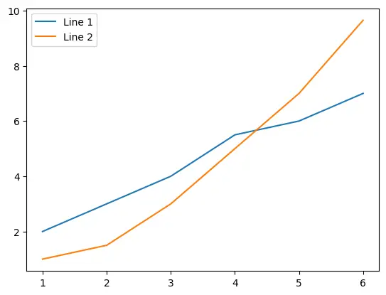
You can also customize other aspects of the legend, such as the location, font size, and more.
Customization of Legends
Matplotlib offers various options to customize the style of legends according to your preferences and create visually appealing plots. In this section, we will focus on some of the frequently used properties that can be adjusted.
1. Modifying Legend Labels
In certain scenarios, it may be necessary to modify the default labels in a legend to accurately represent the plotted data or improve clarity for the viewer. Customizing legend labels becomes particularly useful when dealing with categorical variables or when the default labels lack descriptiveness. To illustrate this, let’s consider an example using a housing dataset that contains information about various features like price, area, number of bedrooms, bathrooms, etc. This dataset enables analysis and exploration of the relationships between these features and the property prices. Firstly, import the required libraries and load the dataset.
import matplotlib.pyplot as plt
import pandas as pd

# Load the housing dataset
df = pd.read_csv('/content/drive/MyDrive/Housing.csv')
In this example, our goal is to create a scatter plot illustrating housing prices based on the area. However, the scatter plot function in Matplotlib requires numeric values for the color parameter, while the “furnishingstatus” column contains textual values. To overcome this, we need to assign a unique numerical value to each category within the “furnishingstatus” column. This mapping process will ensure that each category is represented by a specific numeric value, allowing us to use it as a color parameter in the scatter plot function.
# Map the furnishing status to numeric values for coloring
status_mapping = {'semi-furnished': 0, 'unfurnished': 1, 'furnished': 2}

df['furnishingstatus'] = df['furnishingstatus'].map(status_mapping)
In this particular scenario, the mapping process assigns the values 0, 1, and 2 to the respective categories of ‘semi-furnished’, ‘unfurnished’, and ‘furnished’. This mapping allows us to utilize a specific colormap, such as ‘cool’, to assign distinct colors to the data points in the scatter plot based on their furnishing status.
To create the scatter plot, we use plt.scatter() with ‘area’ for the x-axis and ‘price’ for the y-axis. We then improve readability with labels and a title using plt.xlabel(), plt.ylabel(), and plt.title().
# Plot the scatter plot
scatter = plt.scatter(df['area'], df['price'], c=df['furnishingstatus'], cmap='cool', alpha=0.7)

# Add labels and title
plt.xlabel('Area')
plt.ylabel('Price ($)')
plt.title('Housing Prices')
We then use plt.legend() method to generate the legend for the scatter plot. To achieve this, we pass the handles obtained from the legend elements of the scatter plot using scatter.legend_elements()[0]. By doing so, we ensure that the legend is created based on the distinct values found in the ‘furnishingstatus’ column.
# Define the custom legend labels
legend_labels = ['Semi-Furnished', 'Unfurnished', 'Furnished']

# Create a legend with custom labels
legend = plt.legend(handles=scatter.legend_elements()[0], labels=legend_labels)
To modify the legend labels, we retrieve the legend labels using legend.get_texts() and iterate over them using a loop. Inside the loop, we can customize the labels by setting their font size and color using the set_fontsize(), and set_color() methods.
# Modify the legend labels
labels = legend.get_texts()
for i, label in enumerate(labels):
    label.set_fontsize('small')
    label.set_color('purple')

# Display the plot
plt.show()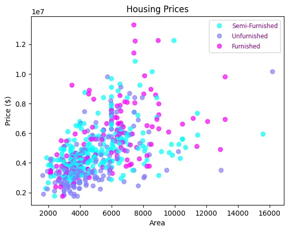
This approach simplifies legend generation by automatically assigning labels based on unique categories in the ‘furnishingstatus’ column. By following this code, you can modify the legend labels in a scatter plot to match your specific requirements.
2. Adjust position Of legend in Python
To adjust the position of the legend in a Matplotlib plot, you can use the loc parameter in the plt.legend() method. This parameter allows you to specify the desired location of the legend. Here are some commonly used loc values to help you position the legend in your plot:
| Values | Description |
| best | Automatically choose the optimal location for the legend. |
| upper left | Place the legend in the upper left corner of the graph. |
| upper right | Place the legend in the upper right corner of the graph. |
| lower left | Place the legend in the lower left corner of the graph. |
| lower right | Place the legend in the lower right corner of the graph. |
| center | Place the legend in the center of the graph. |
| center left | Place the legend in the center-left side of the graph. |
| center right | Place the legend in the center-right side of the graph. |
| upper center | Place the legend in the upper center of the graph. |
| lower center | Place the legend in the lower center of the graph. |
Consider an example of a bar plot to illustrate how to adjust the location of the legend. Suppose we have a dataset that contains the sales performance of different products across multiple months. We want to create a bar plot to visualize the sales for each product and adjust the location of the legend. In this example, we first define the products, months, and sales data.
import matplotlib.pyplot as plt
import numpy as np

# Sample data
products = ['Product A', 'Product B', 'Product C']
months = ['Jan', 'Feb', 'Mar']
sales = np.array([[100, 150, 200],
                  [120, 180, 220],
                  [90, 120, 150]])
We then create a bar plot using a loop to iterate over each product and plot the corresponding sales data using ax.bar(). After that, specify the label parameter in the bar() function to assign labels to each bar.
# Plotting the bar plot
x = np.arange(len(months))
width = 0.2

fig, ax = plt.subplots()
for i, product in enumerate(products):
    ax.bar(x + i*width, sales[i], width, label=product)
To adjust the location of the legend, we use ax.legend(loc='upper left'), where loc specifies the desired location of the legend. By default, the legend is positioned in the upper right corner, but in this case, we have changed its location to the upper left corner to prevent it from overlapping with the data.
# Adjusting the location of the legend
ax.legend(loc='upper left')
The labels to the x-axis and y-axis are assigned using ax.set_xlabel() and ax.set_ylabel(), and ax.set_title() is used to set the title of the plot. Finally, display the plot using plt.show() command.
# Adding labels and title
ax.set_xlabel('Months')
ax.set_ylabel('Sales')
ax.set_title('Product Sales by Month')

# Display the plot
plt.show()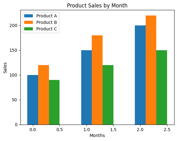
By modifying the loc parameter in the ax.legend() function, you can adjust the location of the legend to different positions, such as ‘upper left’, ‘lower right’, ‘lower left’, or any other desired location.
3. Setting Legend Title
The legend title provides additional context or information about the items represented in the legend. You can set a title for the legend using the set_title() method. This allows you to provide a descriptive title for the legend box. Here’s an example where we use the Iris dataset to create a scatter plot and set a legend title:
import matplotlib.pyplot as plt
import seaborn as sns

# Load the Iris dataset from Seaborn
iris = sns.load_dataset("iris")

# Create a scatter plot
sns.scatterplot(data=iris, x="sepal_length", y="sepal_width", hue="species")

# Add legend with title
legend = plt.legend()
legend.set_title('Flower Species')

# Show the plot
plt.show()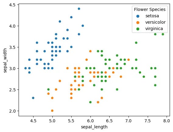
By default, the legend title will be displayed above the legend entries. You can further customize the appearance of the legend title by using additional methods like set_title_fontsize(), set_title_fontweight(), and set_title_fontstyle() to change the font size, weight, and style, respectively.
4. Modifying Legend Box
The legend box in a Matplotlib plot contains the labels and symbols that represent the different elements of the plot, such as lines, markers, or patches. You can customize the appearance of legend box and make it more visually appealing or aligned with the overall style of your plot. For this, we will use the get_frame() method of matplotlib library. Considering the same example as above.
# Set the width of the legend box outline
legend.get_frame().set_linewidth(1.5)

# Set the color of the legend box outline
legend.get_frame().set_edgecolor('blue')

# Set the background color of the legend box
legend.get_frame().set_facecolor('lightgray')

# Show the plot
plt.show()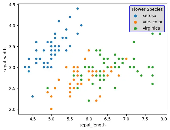
In this example, we use the get_frame method to access the properties of the legend box. We then use the set_linewidth, set_edgecolor, and set_facecolor methods to modify the width, color, and background color of the legend box, respectively.
5. Different Line Styles for Labels
When creating a plot in Matplotlib, it’s common to have multiple lines representing different data or categories. One way to differentiate these lines in the legend is by using different line styles. Matplotlib provides various line styles that can be assigned to each line plot. For example, you can use '-' for a solid line, '--' for a dashed line, ':' for a dotted line, or '-.' for a dash-dot line. By default, Matplotlib assigns the same line style used in the plot to the legend labels. However, if you want to customize the line styles in the legend, you can do so using the lineHandles parameter of the legend() method. This parameter accepts a list of line objects that represent the lines in the legend.
import matplotlib.pyplot as plt
import numpy as np
x = np.linspace(0, 10, 1000)
plt.plot(x, np.sin(x), label='Sine', color='blue', linestyle='-', linewidth=2)
plt.plot(x, np.cos(x), label='Cosine', color='red', linestyle='--', linewidth=2)

# Adding the legend
legend = plt.legend()
legend.set_title('Legend Title')

# Modifying the legend labels
labels = legend.get_texts()
for label in labels:
    label.set_fontsize('small')
    label.set_fontweight('bold')
    label.set_color('green')

legend.get_frame().set_linewidth(1.5)  # Set the width of the legend box outline
legend.get_frame().set_edgecolor('blue')  # Set the color of the legend box outline
legend.get_frame().set_facecolor('lightgray')  # Set the background color of the legend box

# Display the plot
plt.show()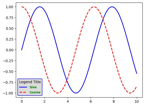
By using different line styles to represent different legend labels, you can visually distinguish between the plotted lines and make it easier for viewers to interpret the graph. Experiment with different line styles to find the combination that best suits your data visualization needs.
Conclusion
In this tutorial, we learned how to add legends to Matplotlib plots in Python. Legends are essential for representing the meaning of different lines or elements in a graph. We explored different ways to customize the appearance of the legend, including modifying the position using the loc parameter and changing the title using the set_title() method. We also discussed how to style the legend and modify the legend box properties. There are several other methods such as adding a shadow effect to the legend boxes or adjusting the spacing between legend handles or labels. We have discussed only few commonly used properties. With these techniques, we can effectively convey the meaning of our plotted data to the viewers of our graphs.
If you want to learn more about matplotlib library and different graphical representations, contact us.